Spectral Algorithms¶

SPy implements various algorithms for dimensionality reduction and supervised & unsupervised classification. Some of these algorithms are computationally burdensome and require iterative access to image data. These algorithms will almost always execute significantly faster if the image data is loaded into memory. Therefore, if you use these algorithms and have sufficient computer memory, you should load your image into memory.

In [1]: from spectral import *

In [2]: img = open_image('92AV3C.lan').load()

Unsupervised Classification¶

Unsupervised classification algorithms divide image pixels into groups based on spectral similarity of the pixels without using any prior knowledge of the spectral classes.

k-means Clustering¶

The k-means algorithm takes an iterative approach to generating clusters. The parameter k specifies the desired number of clusters to generate. The algorithm begins with an initial set of cluster centers (e.g., results from cluster). Each pixel in the image is then assigned to the nearest cluster center (using distance in N-space as the distance metric) and each cluster center is then recomputed as the centroid of all pixels assigned to the cluster. This process repeats until a desired stopping criterion is reached (e.g., max number of iterations). To run the k-means algorithm on the image and create 20 clusters, using a maximum of 50 iterations, call kmeans as follows.

In [3]: (m, c) = kmeans(img, 20, 30)
Initializing clusters along diagonal of N-dimensional bounding box.
Starting iterations.
Iteration 1...done
        21024 pixels reassigned.
Iteration 2...done
        11214 pixels reassigned.
Iteration 3...done
        4726 pixels reassigned.
---// snip //---
Iteration 28...done
        248 pixels reassigned.
Iteration 29...done
        215 pixels reassigned.
Iteration 30...done
        241 pixels reassigned.
^CIteration 31... 15.9%KeyboardInterrupt: Returning clusters from previous iteration

Note that I interrupted the algorithm with a keyboard interrupt (CTRL-C) after the 30th iteration since there were only about a hundred pixels migrating between clusters at that point. kmeans catches the KeyboardInterrupt exception and returns the clusters generated at the end of the previous iteration. If you are running the algorithm interactively, this feature allows you to set the max number of iterations to an arbitrarily high number and then stop the algorithm when the clusters have converged to an acceptable level. If you happen to set the max number of iterations too small (many pixels are still migrating at the end of the final iteration), you can simply call kmeans again to resume processing by passing the cluster centers generated by the previous call as the optional start_clusters argument to the function.

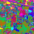
k-means clustering results¶

Notice that kmeans appears to have captured much more of the spectral variation in the image than the single-pass cluster function. Let’s also take a look at the the cluster centers produced by the algorithm:

In [4]: import matplotlib.pyplot as plt

In [5]: plt.figure()

In [6]: for i in range(c.shape[0]):
   ...:     plt.plot(c[i])
   ...: 

In [7]: plt.grid()

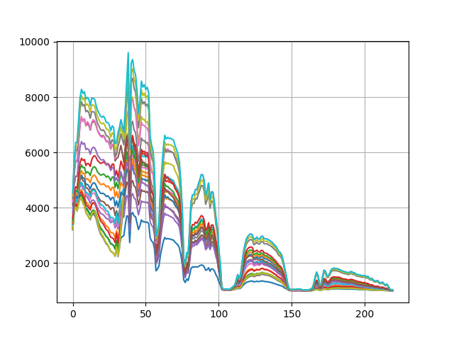
k-means cluster centers¶

Supervised Classification¶

Training Data¶

Performing supervised classification requires training a classifier with training data that associates samples with particular training classes. To assign class labels to pixels in an image having M rows and N columns, you must provide an MxN integer-valued ground truth array whose elements are indices for the corresponding training classes. A value of 0 in the ground truth array indicate an unlabeled pixel (the pixel is not associated with a training class).

The following commands will load and display the ground truth map for our sample image:

In [8]: gt = open_image('92AV3GT.GIS').read_band(0)

In [9]: v = imshow(classes=gt)

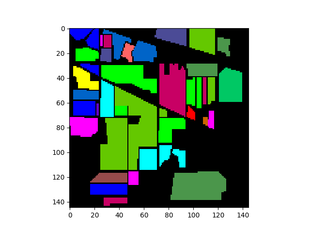
We can now create a TrainingClassSet object by calling create_training_classes:

In [10]: classes = create_training_classes(img, gt)

With the training classes defined, we can then create a supervised classifier, train it with the training classes, and then classify an image.

Gaussian Maximum Likelihood Classification¶

In this case, we’ll perform Gaussian Maximum Likelihood Classification (GMLC), so let’s create the appropriate classifier.

In [11]: gmlc = GaussianClassifier(classes)

When we created the classifier, it was automatically trained on the training sets we provided. Notice that the classifier ignored five of the training classes. GMLC requires computing the inverse of the covariance matrix for each training class. Since our sample image contains 220 spectral bands, classes with fewer than 220 samples will have singular covariance matrices, for which we can’t compute the inverse.

Once the classifier is trained, we can use it to classify an image having the same spectral bands as the training set. Let’s classify our training image and display the resulting classification map.

In [12]: clmap = gmlc.classify_image(img)

In [13]: v = imshow(classes=clmap)

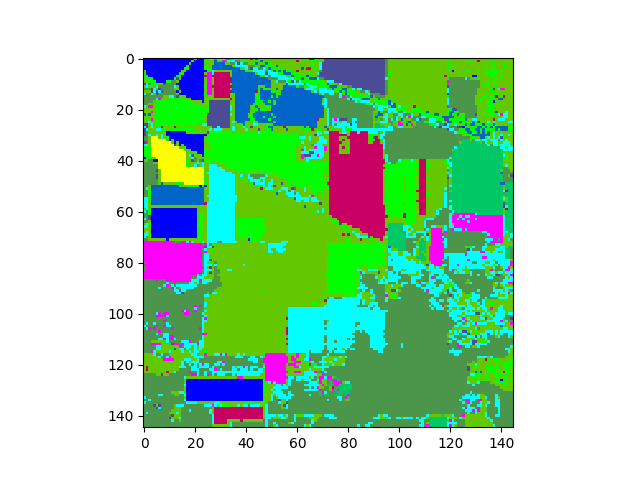
The classification map above shows classification results for the entire image. To view results for only the ground truth pixels we must mask out all the pixels not associated with a training class.

In [14]: gtresults = clmap * (gt != 0)

In [15]: v = imshow(classes=gtresults)

If the classification results are good, we expect the classification map above to look very similar to the original ground truth map. To view only the errors, we must mask out all elements in gtResults that do not match the ground truth image.

In [16]: gterrors = gtresults * (gtresults != gt)

In [17]: v = imshow(classes=gterrors)

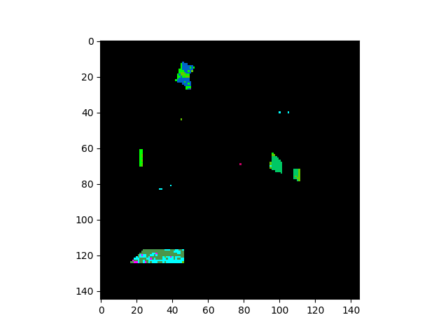
The five contiguous regions in the error image above correspond to the ground truth classes that the GaussianClassifier ignored because they had too few samples.

The following table lists the supervised classifiers SPy currently provides.

Classifier	Description
`GaussianClassifier`	Gaussian Maximum Likelihood
`MahalanobisDistanceClassifier`	Mahalanobis Distance
`PerceptronClassifier`	Multi-Layer Perceptron

Dimensionality Reduction¶

Processing hyperspectral images with hundreds of bands can be computationally burdensome and classification accuracy may suffer due to the so-called “curse of dimensionality”. To mitigate these problems, it is often desirable to reduce the dimensionality of the data.

Principal Components¶

Many of the bands within hyperspectral images are often strongly correlated. The principal components transformation represents a linear transformation of the original image bands to a set of new, uncorrelated features. These new features correspond to the eigenvectors of the image covariance matrix, where the associated eigenvalue represents the variance in the direction of the eigenvector. A very large percentage of the image variance can be captured in a relatively small number of principal components (compared to the original number of bands) .

The SPy function principal_components computes the principal components of the image data and returns the mean, covariance, eigenvalues, and eigenvectors in a PrincipalComponents. This object also contains a transform to rotate data in to the space of the principal compenents, as well as a method to reduce the number of eigenvectors.

In [18]: pc = principal_components(img)

In [19]: v = imshow(pc.cov)

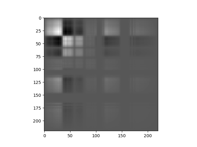
In the covariance matrix display, whiter values indicate strong positive covariance, darker values indicate strong negative covariance, and grey values indicate covariance near zero.

To reduce dimensionality using principal components, we can sort the eigenvalues in descending order and then retain enough eigenvalues (an corresponding eigenvectors) to capture a desired fraction of the total image variance. We then reduce the dimensionality of the image pixels by projecting them onto the remaining eigenvectors. We will choose to retain a minimum of 99.9% of the total image variance.

In [20]: pc_0999 = pc.reduce(fraction=0.999)

In [21]: # How many eigenvalues are left?

In [22]: len(pc_0999.eigenvalues)
Out[22]: 32

In [23]: img_pc = pc_0999.transform(img)

In [24]: v = imshow(img_pc[:,:,:3], stretch_all=True)

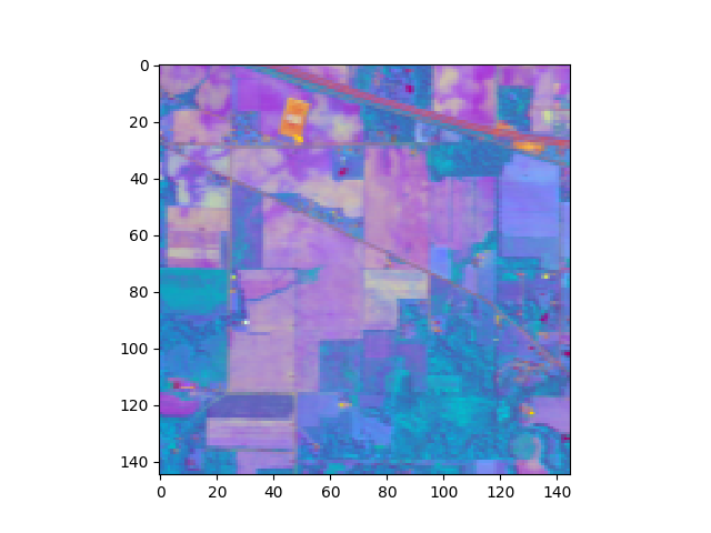
Now we’ll use a Gaussian maximum likelihood classifier (GMLC) for the reduced principal components to train and classify against the training data.

In [25]: classes = create_training_classes(img_pc, gt)

In [26]: gmlc = GaussianClassifier(classes)

In [27]: clmap = gmlc.classify_image(img_pc)

In [28]: clmap_training = clmap * (gt != 0)

In [29]: v = imshow(classes=clmap_training)

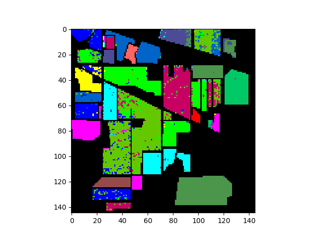
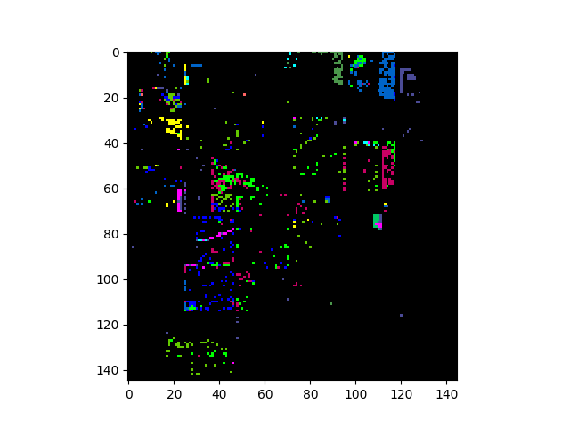
And the associated errors:

In [30]: training_errors = clmap_training * (clmap_training != gt)

In [31]: v = imshow(classes=training_errors)

Fisher Linear Discriminant¶

The Fisher Linear Discriminant (a.k.a., canonical discriminant) attempts to find a set of transformed axes that maximize the ratio of the average distance between classes to the average distance between samples within each class. [Richards1999] This is written as

$C_b x = \lambda C_w x$

where $C_b$ is the covariance of the class centers and $C_w$ is the weighted average of the covariances of each class. If $C_w$ is invertible, this becomes

$\left(C_{w}^{-1} C_b\right)x=\lambda x$

This eigenvalue problem is solved by the linear_discriminant function, yielding C-1 eigenvalues, where C is the number of classes.

In [32]: classes = create_training_classes(img, gt)

In [33]: fld = linear_discriminant(classes)

In [34]: len(fld.eigenvectors)
Out[34]: 220

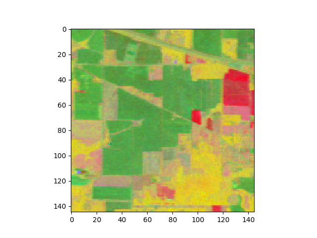
Let’s view the image projected onto the top 3 components of the transform:

In [35]: img_fld = fld.transform(img)

In [36]: v = imshow(img_fld[:, :, :3])

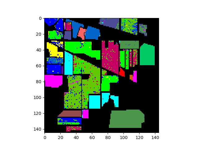
Next, we’ll classify the data using this discriminant.

In [37]: classes.transform(fld.transform)

In [38]: gmlc = GaussianClassifier(classes)

In [39]: clmap = gmlc.classify_image(img_fld)

In [40]: clmap_training = clmap * (gt != 0)

In [41]: v = imshow(classes=clmap_training)

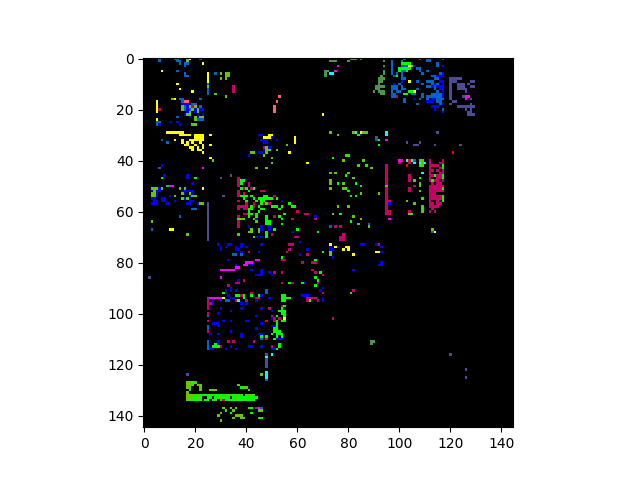
In [42]: fld_errors = clmap_training * (clmap_training != gt)

In [43]: v = imshow(classes=fld_errors)

Target Detectors¶

RX Anomaly Detector¶

The RX anomaly detector uses the squared Mahalanobis distance as a measure of how anomalous a pixel is with respect to an assumed background. The SPy rx function computes RX scores for an array of image pixels. The squared Mahalanobis distance is given by

$y=(x-\mu_b)^T\Sigma_b^{-1}(x-\mu_b)$

where $x$ is the pixel spectrum, $\mu_b$ is the background mean, and $\Sigma_b$ is the background covariance [Reed_Yu_1990].

If no background statistics are passed to the rx function, background statistics will be estimated from the array of pixels for which the RX scores are to be calculated.

In [44]: rxvals = rx(img)

To declare pixels as anomalous, we need to specify a threshold RX score. For example, we could choose all image pixels whose RX score has a probability of less than 0.001 with respect to the background:

In [45]: from scipy.stats import chi2

In [46]: nbands = img.shape[-1]

In [47]: P = chi2.ppf(0.999, nbands)

In [48]: v = imshow(1 * (rxvals > P))

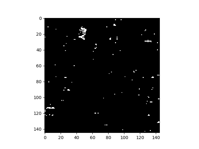
Rather than specifying a threshold for anomalous pixels, one can also simply view an image of raw RX scores, where brighter pixels are considered “more anomalous”:

In [49]: v = imshow(rxvals)

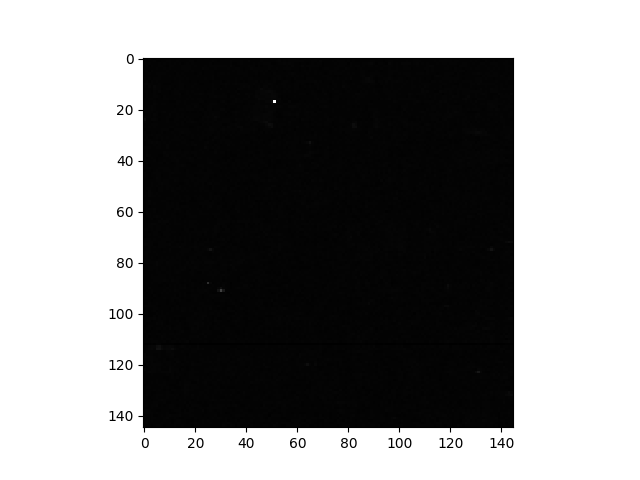
For the sample image, only a few pixels are visible in the image of RX scores because a linear color scale is used and there is a very small number of pixels with RX scores much higher than other pixels. This is apparent from viewing the histogram of the RX scores.

In [50]: import matplotlib.pyplot as plt

In [51]: f = plt.figure()

In [52]: h = plt.hist(rxvals.ravel(), 200, log=True)

In [53]: h = plt.grid()

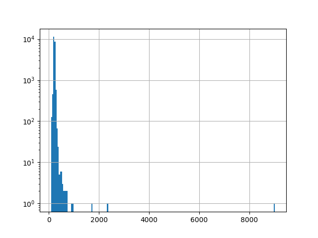
The outliers are not obvious in the histogram, so let’s print their values:

In [54]: print(np.sort(rxvals.ravel())[-10:])
[ 665.17211462  675.85801536  683.58190673  731.4872873   739.95211335
  906.98669373  956.49972325 1703.20957949 2336.11246149 9018.65517253]

To view greater detail in the RX image, we can adjust the lower and upper limits of the image display. Since we are primarily interested in the most anomalous pixels, we will set the black level to the 99th percentile of the RX values’ cumulative histogram and set the white point to the 99.99th percentile:

In [55]: v = imshow(rxvals, stretch=(0.99, 0.9999))

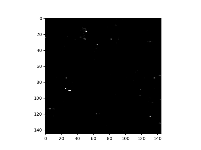
We can see the new RGB data limits by inspecting the returned ImageView object:

In [56]: print(v)
ImageView object:
  Display bands       :  [0]
  Interpolation       :  <default>
  RGB data limits     :
    R: [291.6938067178437, 956.4997232540622]
    G: [291.6938067178437, 956.4997232540622]
    B: [291.6938067178437, 956.4997232540622]

Note that we could also have set the contrast stretch to explicit RX values (vice percentile values) by specifying the bounds keyword instead of stretch.

If an image contains regions with different background materials, then the assumption of a single mean/covariance for background pixels can reduce performance of the RX anomaly detector. In such situations, better results can be obtained by dynamically computing background statistics in a neighborhood around each pixel being evaluated.

To compute local background statistics for each pixel, the rx function accepts an optional window argument, which specifies an inner/outer window within which to calculate background statistics for each pixel being evaluated. The outer window is the window within which background statistics will be calculated. The inner window is a smaller window (within the outer window) indicating an exclusion zone within which pixels are to be ignored. The purpose of the inner window is to prevent potential anomaly/target pixels from “polluting” background statistics.

For example, to compute RX scores with background statistics computed from a 21 $\times$ 21 pixel window about the pixel being evaluated, with an exclusion window of 5 $\times$ 5 pixels, the function would be called as follows:

In [57]: rxvals = rx(img, window=(5,21))

While the use of a windowed background will often improve results for images containing multiple background materials, it does so at the expense of introducing two issues. First, the sizes of the inner and outer windows must be specified such that the resulting covariance has full rank. That is, if $w_{in}$ and $w_{out}$ represent the pixel widths of the inner and outer windows, respectively, then $w_{out}^2 - w_{in}^2$ must be at least as large as the number of image bands. Second, recomputing the estimated background covariance for each pixel in the image makes the computational complexity of of the RX score computation orders of magnitue greater.

As a compromise between a fixed background and recomputation of mean & covariance for each pixel, rx can be passed a global covariance estimate in addition to the window argument. In this case, only the background mean within the window will be recomputed for each pixel. This significanly reduces computation time for the windowed algorithm and removes the size limitation on the window (except that the outer window must be larger than the inner). For example, since our sample image has ground cover classes labeled, we can compute the average covariance over those ground cover classes and use the result as an estimate of the global covariance.

In [58]: C = cov_avg(img, gt)

In [59]: rxvals = rx(img, window=(5,21), cov=C)

Matched Filter¶

The matched filter is a linear detector given by the formula

$y=\frac{(\mu_t-\mu_b)^T\Sigma_b^{-1}(x-\mu_b)}{(\mu_t-\mu_b)^T\Sigma^{-1}(\mu_t-\mu_b)}$

where $\mu_t$ is the target mean, $\mu_b$ is the background mean, and $\Sigma_b$ is the covariance. The matched filter response is scaled such that the response is zero when the input is equal to the background mean and equal to one when the pixel is equal to the target mean. Like the rx function the SPy matched_filter function will estimate background statistics from the input image if no background statistics are specified.

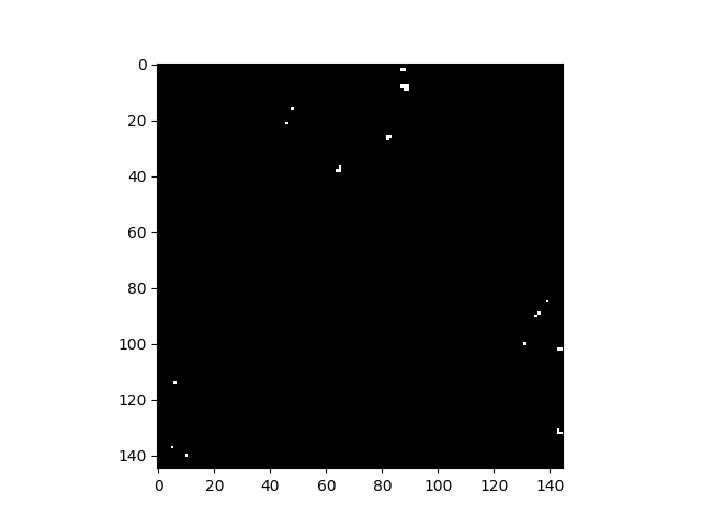
Let’s select the image pixel at (row, col) = (8, 88) as our target, use a global background statistics estimate, and plot all pixels whose matched filter scores are greater than 0.2.

In [60]: t = img[8, 88]

In [61]: mfscores = matched_filter(img, t)

In [62]: v = imshow(1 * (mfscores > 0.2))

As with the rx function, matched_filter can be applied using windowed background statistics (optionally with a global covariance estimate).

Miscellaneous Functions¶

Band Resampling¶

Comparing spectra measured with a particular sensor to spectra collected by a different sensor often requires resampling spectra to a common band discretization. Spectral bands of a single sensor may drift enough over time such that spectra collected by the same sensor at different dates requires resampling.

For resampling purposes, SPy treats a sensor as having Gaussian spectral response functions for each of its spectral bands. A source sensor band will contribute to any destination band where there is overlap between the FWHM of the response functions of the two bands. If there is an overlap, an integral is performed over the region of overlap assuming the source band data value is constant over its FWHM (since we do not know the true spectral load over the source band) and the destination band has a Gaussian response function. Any target bands that do not have an overlapping source band will produce NaN as the resampled band value. If FWHM information is not available for a sensor’s bands, each band’s FWHM is assumed to reach half the distance the its adjacent bands. Resampling results are better when source bands are at a higher spectral resolution than the destination bands.

To create BandResampler object, we can either pass it a BandResampler object for each sensor or a list of band centers and, optionally, a list of FWHM values. Once the BandResampler is created, we can call it with a source sensor spectrum and it will return the resampled spectrum.

In [63]: import spectral.io.aviris as aviris

In [64]: img1 = aviris.open('f970619t01p02_r02_sc04.a.rfl', 'f970619t01p02_r02.a.spc')

In [65]: bands2 = aviris.read_aviris_bands('92AV3C.spc')

In [66]: resample = BandResampler(img1.bands, bands2)

In [67]: x1 = img1[96, 304]

In [68]: x2 = resample(x1)

NDVI¶

The Normalized Difference Vegetation Index (NDVI) is an indicator of the presence of vegetation. The index is commonly defined as

$NDVI = \frac{NIR-RED}{NIR+RED}$

where NIR is the reflectance in the near infrared (NIR) part of the spectrum and RED is the reflectance of the red band. For our sample image, if we take band 21 (607.0 nm) for our red band and band 43 (802.5 nm) for near infrared, we get the following NDVI image.

In [69]: vi = ndvi(img, 21, 43)

In [70]: v = imshow(vi)

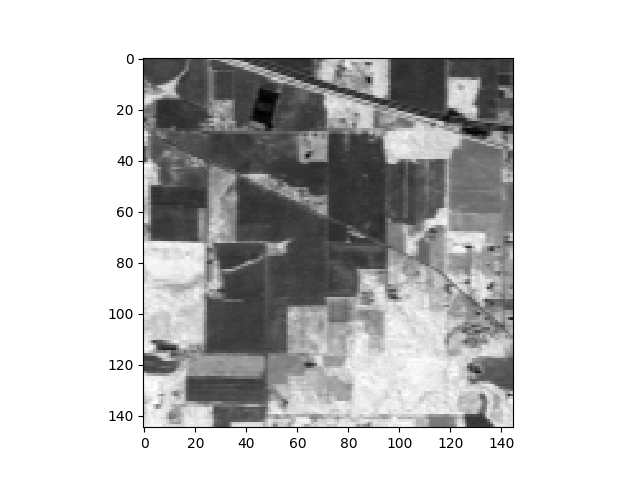
ndvi is a simple convenience function. You could just as easily calculate the vegetation index yourself like this:

In [71]: red = img.read_band(21)

In [72]: nir = img.read_band(43)

In [73]: vi = (nir - red) / (nir + red)

Spectral Angles¶

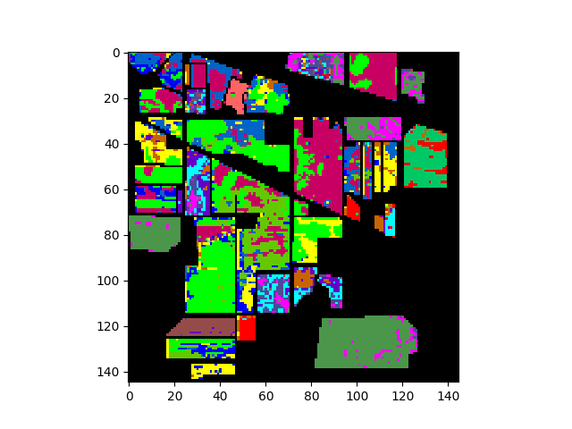
A spectral angle refers to the angle between to spectra in N-space. In the absence of covariance data, spectral angles can be used for classifying data against a set of reference spectra by selecting the reference spectrum with which the unknown spectrum has the smallest angle.

To classify our sample image to the ground truth classes using spectral angles, we must compute the spectral angles for each pixel with each training class mean. This is done by the spectral_angles function. Before calling the function, we must first create a CxB array of training class mean spectra, where C is the number of training classes and B is the number of spectral bands.

In [74]: import numpy as np

In [75]: classes = create_training_classes(img, gt, True)

In [76]: means = np.zeros((len(classes), img.shape[2]), float)

In [77]: for (i, c) in enumerate(classes):
   ....:     means[i] = c.stats.mean
   ....: 

In the code above, the True parameter to create_training_classes forces calculation of statistics for each class. Next, we call spectral_angles, which returns an MxNxC array, where M and N are the number of rows and columns in the image and there are C spectral angle for each pixel. To select the class with the smallest angle, we call the numpy argmin function to select the index for the smallest angle corresponding to each pixel. The clmap + 1 is used in the display command because our class IDs start at 1 (not 0).

In [78]: angles = spectral_angles(img, means)

In [79]: clmap = np.argmin(angles, 2)

In [80]: v = imshow(classes=((clmap + 1) * (gt != 0)))